Outline thermal behaviour of metallic conductors

1. Executive Summary
   

   Faraday asserted the economic optimum of a conductor with balanced costs of resistive dissipation and finance. This is simple to prove for an unprotected cable with fixed resistivity but variations in resistivity from temperatures caused by current loads and the  impacts from short-circuits and over-loads need to be included in any detailed engineering study of the loading, behaviours and protection of electrical-power conductors and their connections

   The calculations and Finite Element Analysis (FEA) results included below are taken from a paper written by Christopher Langridge, from LML Products and Riker, in collaboration with Dr Joan Lasenby, of Trinity College Cambridge, and presented at the 2015 Railway Engineering Conference.

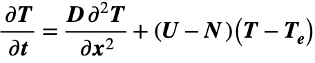
   FEA models had originally been set up to examine the thermal performance of crimped terminations on cables of various sizes as a precursor to thermal-cycle and surge-current endurance tests. The observed behaviour differences between stable load-currents and near-adiabatic surge currents led to the formulation of a Central Differential Equation (CDE) whose solutions predicted basic behaviour patterns. It explains and predicts the effect of load current and resistive heating, dependent on load current, geometry, conductor properties and external conditions. These predictions were validated, to high accuracy, by further FEA studies which used basic physical properties only and did not incorporate the CDE’s formulation or solutions.
   

   The investigation applied to copper but has similar application to aluminium or other metals. 

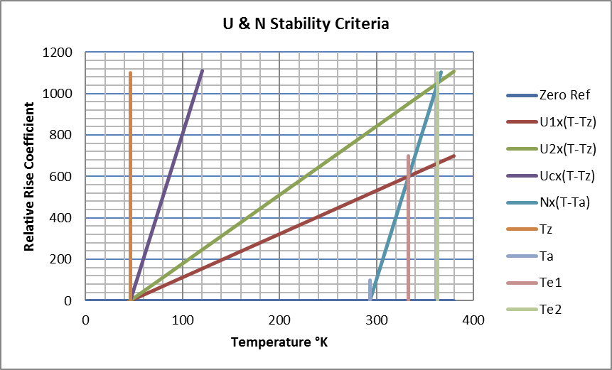
   The CDE model is based on two main properties of conductors; their coefficient of resistive heating, U, and their coefficient of surface cooling, N. Results can be summarised with reference to the graphic showing the Conditions for Stable Working Temperatures, U & N Stability Criteria which illustrates two main effects of increasing conductor temperature:

   1. An increase in electrical resistivity which can be taken as linear with respect to temperature above an originating zero-point temperature, Tz, (ITRO -227°C for copper) and increases resistive  heating  to a value of U x (T-Tz) at Temperature = T within a given cable under given load-current. The graphic shows two stable cases of cables plus load-currents, given by U1 x (T-Tz) & U2 x (T-Tz), plus a critical-instability case, given by Uc x (T-Tz).
   2. An increase in (Newtonian) surface thermal dissipation, taken as linear with respect to temperature above the ambient air, Ta, to give the value shown on the graphic of N x (T-Ta) at Temperature = T. The cooling-process (diffusion, convection, forced-air) and conductor surface-area determine N and the consequent rate of heat loss.

      These two effects combine to provide two basic behaviours:

      Stable Behaviour
      

      Starting from ambient (and therefore zero cooling) the temperature of a current-loaded conductor will rise until bulk resistive heating balances surface thermal dissipation at an Equilibrium Temperature shown with two cases on the graphic at Te1 and Te2.

      Load-currents causing resistive heating below the critical level, Uc x (T-Tz), produce benign thermal behaviour characterised by rate-determined asymptotic approaches to stable temperatures over time and distance at characteristic convergence rates. Uniform conductors have only time-dependent convergence.  High metallic thermal-conductivity prevents significant temperature excursions at small regions of restriction and allows extended smooth axial variations in temperature between differing but lightly-loaded cables. Forced temporary temperature excursions under equilibrium conditions (e.g. caused by local external heating or previous surge-current events) revert to normal convergence to equilibrium when the unusual influence is removed. 

      These stable behaviours, with respect to both time and axial distance along the conductor, are described by a set of solutions to the CDE comprising convergent exponential functions which provide an asymptotic approach to stability over both axial distance along the conductor and time. They are illustrated by the FEA results shown in the text below with Figs 02a-c.

      Unstable Behaviour
      

      If the load-current within a conductor of given geometry is increased, then the line describing resistive heating increases in gradient and above a critical level, Uc x (T-Tz), is unable to intercept the line, N x (T-Ta), describing heat-loss. The rate of increase in resistive heating with temperature now exceeds the corresponding increase in available cooling. Stable temperature equilibrium is no longer possible and temperature rise becomes inexorable. 

      Bulk thermal conductivity within the conductor is now unable to disperse localised excess resistive heating and restrictions in the conductor can therefore cause severe rapid temperature excursions. Externally imposed irregularities in the temperature distribution are also exacerbated to become amplified local singularities.

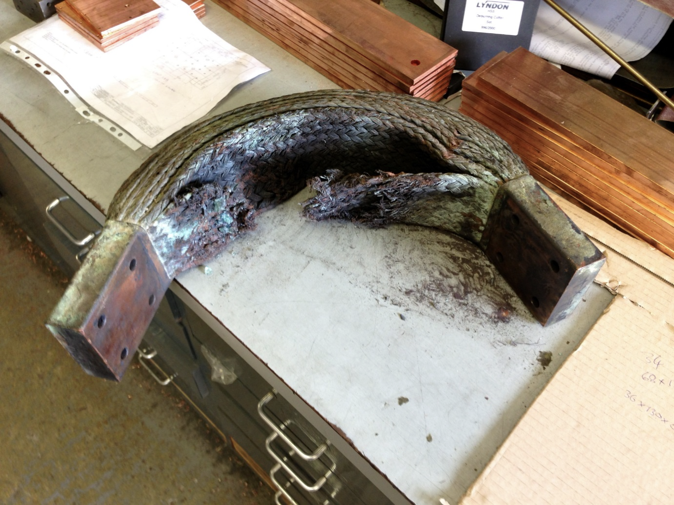
      The structure also describes localised destructive failures (as opposed to extended uniform melting) frequently observed in cables and conductors subjected to extreme overloads. Picture 01, below, shows a conductor constructed from multiple braids consolidated into a right-angle-bend connection. There is very poor lateral thermal transfer between the braids and the shortest path length of the inside braid will have increased its working current-density and temperature; particularly at its mid-point between the uniform lower temperatures of the two terminations. Under overload conditions this results in early failure of the inner braid near its centre; note the localisation of damage.

      Picture 01: Localised Destructive Failure in Flexible Power Connector
      
      

      These behaviours are described by solutions to the CDE where the conditions required for stability are exceeded and its convergent asymptotic solutions are no longer applicable. Available solutions now comprise a combination of divergent exponentials with respect to time (with positive-real exponential coefficients) and wave functions with respect to distance (with complex-number exponential coefficients). Under equilibrium conditions, axial temperature waves externally imposed onto the conductor would disperse over time as thermal conductivity is adequate to disperse the temperature gradients carrying excess heat generated at peak temperature points to the troughs between them. Under extreme conditions outside equilibrium however, thermal conduction to adjacent troughs is inadequate to arrest the acceleration of peak temperatures. Increasing the current level supports shorter spatial wavelengths with higher thermal gradients; temperature singularities with smaller dimensions are then exacerbated over time. These particular wave-dispersion or exacerbation phenomena were investigated and verified in detail by various FEA time-study models where wave-structures were initiated over axial distance or injected over time. 

      The FEA models used only axial temperature variations within long conductors, treated as solid, with variations in cross-sectional area. Individual elements comprised small axial divisions of the conductor which were taken to have only axial temperature variation and trans-axial temperature variations were ignored. Independent variables were therefore restricted to time one spatial dimension. This was however adequate to confirm the CDE predictions of interest to a high level of accuracy; as revealed in the main text below. It also enabled further accurate modelling of the behaviour of solid cable terminations fixed onto cables with local solidification from crimp-fastening the termination. Results from these models are not described in this text. Details relating to stranded cables and their internal temperature distribution would require more complex modelling. 

      The Central Differential Equation provides a valuable insight into details of the basic stable and unstable behaviours described. Apart from cases involving uniform conductors and simple geometric forms however, analytic applications of the CDE are probably rare. Finite Element Analysis, used here for detailed behaviour verification, provides the main resource for investigating complex engineering installations and the behaviours illuminated by the CDE.

2. Physical Model 

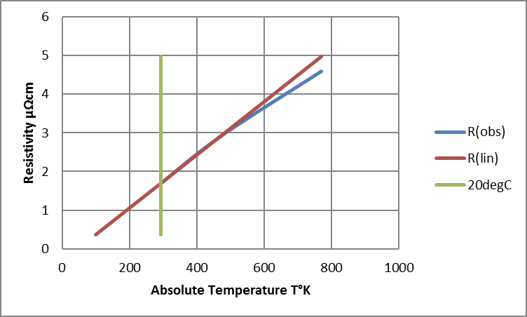
   Being temperature-dependent, values for internal electrical resistivity, internal thermal conductivity and external thermal dissipation need calculating for each element as it tracks its temperature trajectory. Examination of physically determined values showed that, over the working range of interest (say, -200 to +500°C), variations in electrical resistivity (Fig 01) and thermal conductivity were satisfactorily modelled by linear variations in temperature. (Outside this range, the model was still valid in terms of the defined physical properties but might differ from real life owing to second-order effects which effectively provided a different, but corresponding, temperature scale.) Qualitatively, an increase in temperature increases electrical resistance through dynamic metal lattice distortion; electrically conductive electrons are impeded by interaction with an increase in lattice vibration phonons. (Note also that an impurity, such as tin in copper, results in a static lattice distortion that has a similar detrimental effect on resistance. A given concentration of impurity adds a fixed resistance that is equivalent to adding a fixed temperature offset into the determination of temperature-dependent variation.) Both phonons and electrons contribute to thermal conductivity however and the increase in detrimental electron-phonon and phonon-phonon interactions is partially restored by an increase in phonon population and energy. For copper, electrical resistivity was taken to increase by 0.4% per °C and thermal conductance was taken to reduce by 0.014% per °C. This latter is equivalent to an increase in thermal resistivity of 0.014% per °C and about 1/30^th the variation rate for electrical resistivity 

   Fig 01: Observed and Linear-Modelled Variations in Resistivity
   
   

   Thermal Dissipation by Diffusion and Convection (Natural or Forced)

   The Newtonian cooling model proportions heat loss from external surface area against temperature difference over ambient with an environmental cooling factor. Newtonian Heat Transfer Coefficients (NHTCs) for air cooling, in Wm^-2K^-1, can be anywhere between 0.5-1000 but typically have values ITRO 2-35 for convection. 

   Levels ITRO 0.5 Wm^-2K^-1correspond to diffusion without bulk air movement when temperature differentials are low or air-flow is restricted.

   Quoted Thermal Resistance values for natural convection with small finned heat-sinks correspond to NHTC values ITRO 6-8 Wm^-2K^-1.

   Air moving at 5 ms¯¹ (11mph) provides an NHTC value ITRO 25 Wm^-2K^-1. 

3. Initial Finite Element Abnalysis

   The issue remaining was to look at how a system of conductors and connectors might be analysed in terms of useful mathematical models of its component parts. The differential equations governing overall behaviour could be readily assembled but they could only be expected to cover a defined uniform region of space. Real-life problems involve more elaborate geometry and, with few exceptions, are unlikely to be described by an obliging function neatly fitting the boundary conditions of a closely defined space. A pragmatically universal solution requires multiple elemental regions. Each element can then sustain a smooth solution that matches state and flux boundary conditions with each adjacent partner or outer surface.

   The principal aim of FEA modelling was to establish the effects of geometry, conductor mass and current loading on the temperature distribution along the bulk features of conductors and connections. This was intended to optimise design specifications and parameters for test survival and field reliability. Initial physical measurements had already shown that, with normal working current densities, the high thermal conductivity of copper (or aluminium) enabled the bulk conductor to very effectively restrain local temperature excursions at any point of reduced cross-section. Internal trans-axial distributions of temperature within the conductor were not, therefore, being considered at this stage. In fact, a simple one-dimensional finite-element model was used to assess temperature distributions in bus-bars, cables and terminations.

   Confining the model to one spatial dimension plus time clearly simplifies the calculation process; cable and connector elements are generally modelled as linked cone frusta with matching cross-sections at each interface. Newtonian cooling provides surface dissipation into a fixed ambient with elected cooling constant. This simple concept can be readily modified, wherever required, to accommodate the attributes of real-life surface and cross-section geometry. For example, transitions to square or tubular section can be modelled simply on the basis of their surface and cross-section areas. Otherwise, any cone angle should, ideally, be kept small in order to simplify accurate modelling of heat flux and surface dissipation.

   With geometric and material factors now covered, a defined time increment enabled the temperature rise for each iteration step to be simply calculated from net conducted and dissipated heat flux plus resistive heating. It did prove necessary, however, to reduce iteration step-time in concert with either improved axial resolution or increased load current. This was taken to indicate the need for workable first-order temperature variation between iterations in time without significant effects from variations of second-order or above.

   In fact, maintaining linearity in charts of evolving dθ/dt and d²θ/dt² proved to be a simple valuable “dashboard indication” of stability for a chosen iteration time increment. The measurements of first and second time-derivatives also provided a running check on convergence/divergence time constant, plus predicted asymptote, for different regions of a given model.

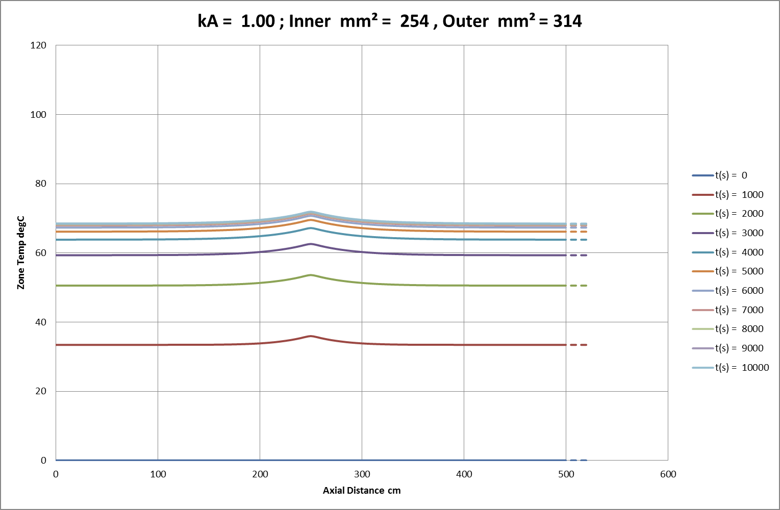
   Fig 02a: Initial FEA Result for 81% Cross-Section over 250cm of 500cm Conductor; Amb. = 0°C.

   

   
   

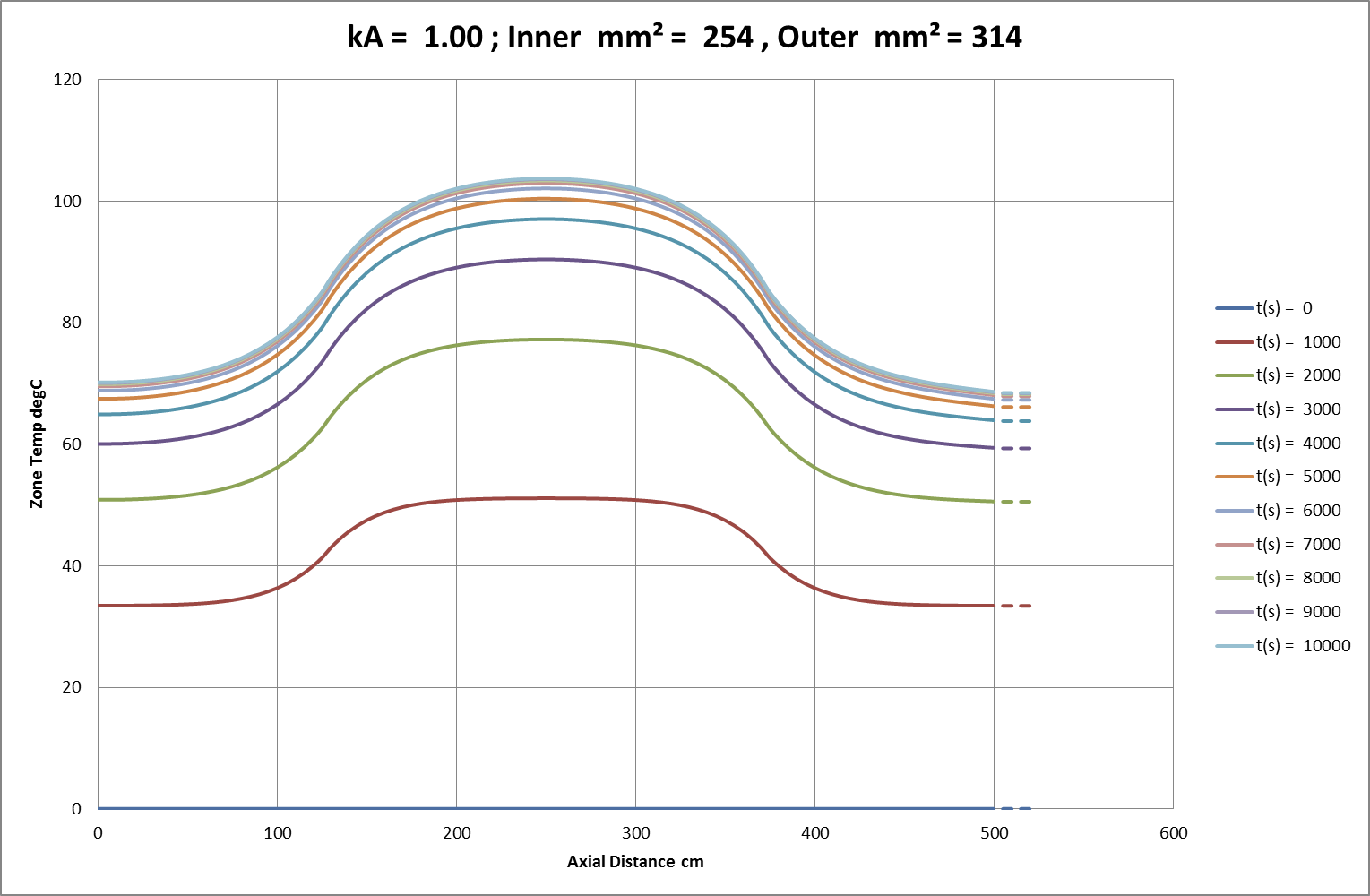
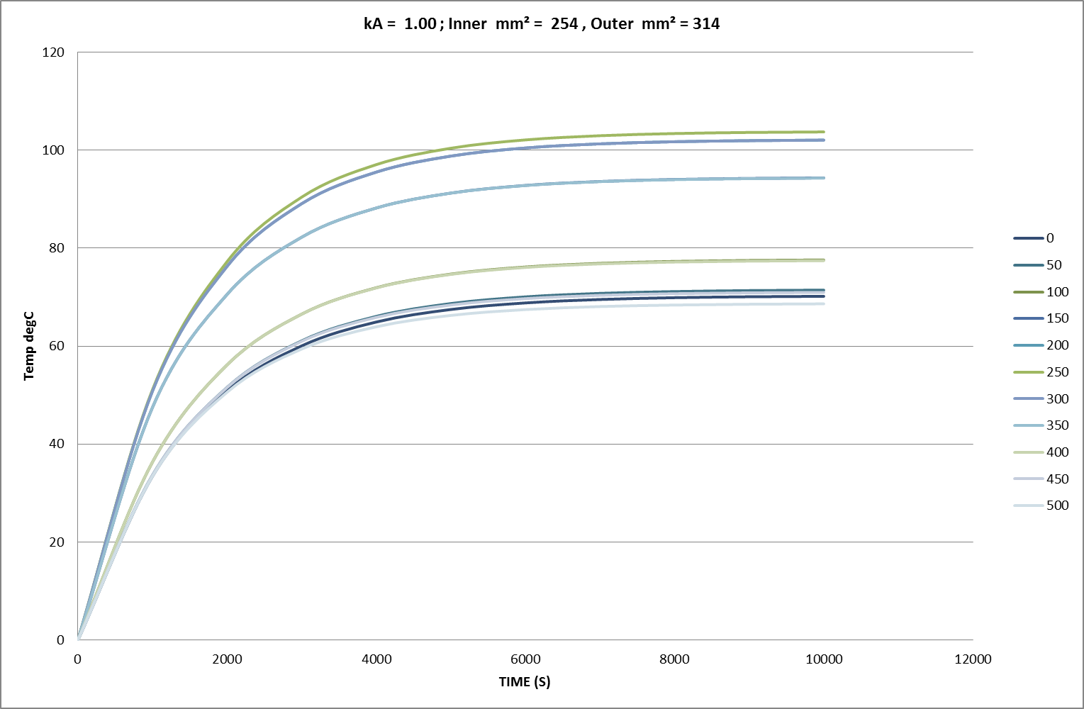
   Fig 02b: Initial FEA Result for 81% Cross-Section over 25cm of 500cm Conductor; Amb. = 0°C.

   

   

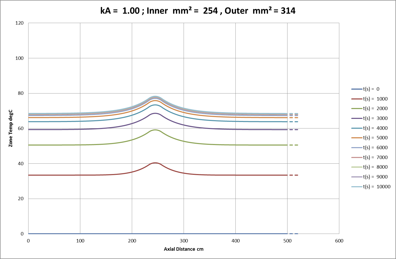
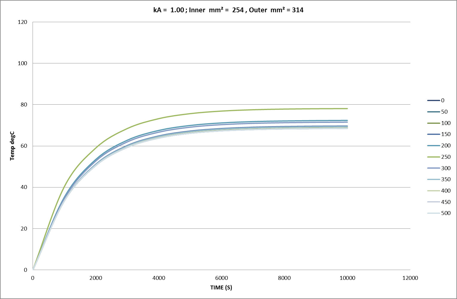
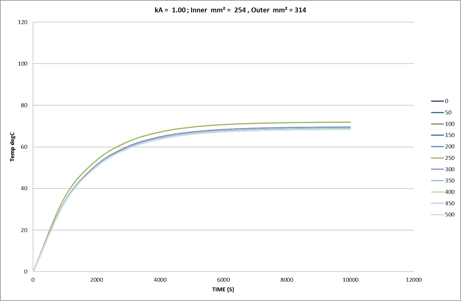
   Fig 02c: Initial FEA Result for 81% Cross-Section over 5cm of 500cm Conductor; Amb. = 0°C.

   

   

   Initial FEA Results

   Using “working” current densities, Figs 02a-c show the familiar characteristic convergence, over time and distance, towards finite temperature asymptotes. In these charts the squared current density ratio is 153%, closely matching the observed ratio of temperature asymptotes in Fig 02a. Axial thermal conduction impacts significantly on overall heat distribution and dissipation. In line with this behaviour, small regions of reduced cross-section are heavily restrained by the larger regions of adjacent conductor. Finally, other tests showed that any initial axial deviations or time-dependent variations from the equilibrium temperature distribution rapidly dissolved into these asymptotic uniformities. The results of more detailed measurements follow later in the text.

   When the simulations were extended to very high current densities (corresponding to surge-currents with temperature rise-rates in the region of 100degC/sec) a rather different set of behaviours started to appear in the models. Once current exceeded a “critical” value, temperatures would not stabilise but increase exponentially as each temperature increment caused an increase in resistive heating that exceeded the increase in Newtonian cooling.

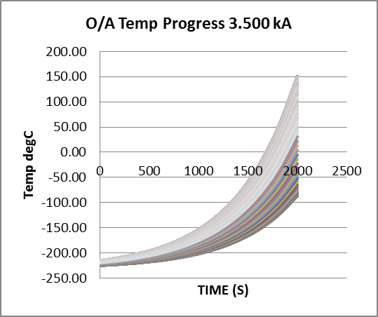
   Fig 03: Exponential Temperature Rise to Melting in c. 1.2s.
   
   

   This was, again, much as expected but it was also noticed that, in place of dissipation and dependent upon current, some temperature patterns could also become unstable. In other words, local regions of higher temperature might grow in size and extent rather than simply diffuse and disperse. This pointed toward the emergence of “parasitic” temperature distributions superimposed on an overall trajectory.

   Obviously, such behaviour has the potential to affect the duty-cycle stresses and survival of a whole spectrum of electrical systems. It was, therefore, felt relevant to explore, map and measure FEA results in comparison with predictions from mathematical analysis.

4. Central Differential Equation and Solutions
   

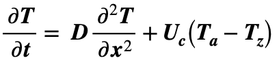
   The basic equation describing temperature is based on a conductor element of length l with perimeter p and cross-section A. The element carries a current u (u  is being used for current to avoid confusion with the imaginary number, i) and is surrounded by an environment at ambient temperature T_a.

   The rate of temperature increase is now dependent upon the following main factors:

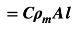
   The thermal mass of the element = Specific Heat x Density x Volume
   

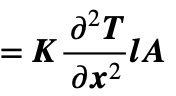
   The internal resistive heat generation = (Current)² x Resistance
   

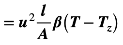
        [ B is the factor proportioning resistivity to its effective linear zero = T_z   , see above.]

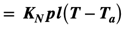
   The external heat dissipation = (Cooling Factor) x (Surface Area) x (Temp over Ambient)
   

   The net conducted heat flux = (Therm Cond) x (RoC [Temp Grad] x Length) x (Cross-Section)
   

   After normalising volume,the rate of temperature rise is therefore given by a central differential equation (CDE):
   

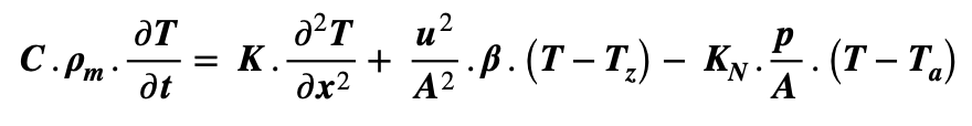
   Simplifying the above yields:
   
   

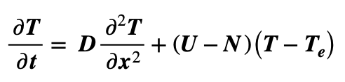
   (Note: care required for cases where U = N .)

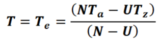
   Making the substitution Z = (T – T_e)  now gives a simplified version of the CDE:
   

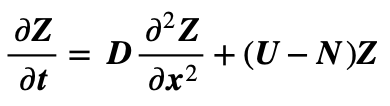
   So that separation of variables then yields solutions of the form:
   

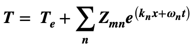
   Note, at this stage, that the linearity of Z within the CDE means that separate solutions, each satisfying the CDE and CSE, can be superposed. If and are both solutions to 104 then their sum  Z_s ( = Z₁ + Z₂)  is also a solution. In fact, the solution for Z is a sum of all possible individual solutions.  After re-substituting T_e, T is therefore now given by:
   
   

    

   A sum of solutions for Z plus an offset temperature, T_e, the total of which must conform to the imposed boundary conditions. Substituting a given solution for Z back into the simplified CDE now gives a Central State Equation (CSE) for w and k. Any one solution complies with the CSE as follows:

   

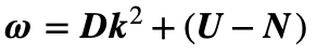
   This describes the balance between spatial and temporal time constants for the thermal mass under the influence of U (variation of resistive heating with temperature) and N (variation of Newtonian cooling with temperature). Remember however that this applies to the Z portion of temperature; i.e. without any offset. Immediately obvious from the CSE is the parabolic relationship between real values for w and k when  w – (U – N) ≥ 0. Also clear from the CSE is the situation where U < N and K ~0   to give w < 0 in (106) with temperature converging towards equilibrium at T = T_e.

   Fig 04: Conditions for Stable Working Temperatures
   
   

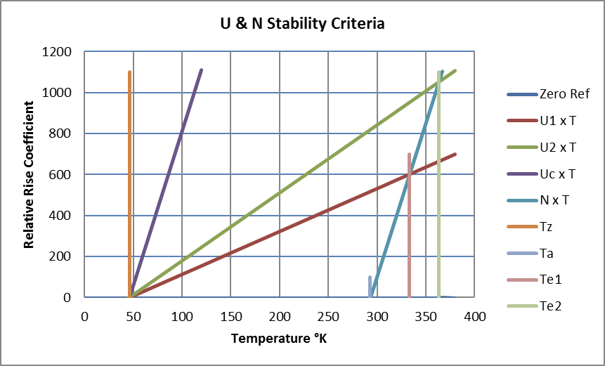
   Stable working temperatures require:

   1. T_a > T_z : The ambient is greater than the resistive zero-reference temperature. 
   2. U < N : Any temperature rise yields a net increase in cooling over resistive heating. 

   Over time, this enables an asymptotic approach to an equilibrium temperature with positive or negative real values of k fitting thermal gradients between boundary temperature values.
   

   Referring back to the simplified CDE, , stability in a uniform conductor is possible with zero values for both temporal and spatial variations in temperature so that
        

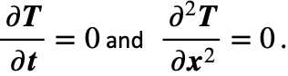
   For a non-zero current with U < N, equilibrium is reached at the temperature shown in (103):

   

   Effect of Impurities

   Impurities such as tin, when introduced into the copper conductor matrix, generally impose a fixed lattice disorder corresponding to a fixed temperature offset in the resistance characteristic. The incremental change in resistance with temperature remains unchanged. This does not affect the ability to reach equilibrium, but it will significantly increase both the resistance at any temperature and the ultimate equilibrium temperature. It is perfectly possible, through diffusion of coatings, to introduce 1% tin into finely stranded copper cables. This increases the resistivity of copper at 20°C by a factor of about 2.5 with the apparent linear offset temperature ( T_z ) consequently moving from about -227°C (46°K) to about -600°C (-327°K).

   Critical Boundary and Incipient Instability

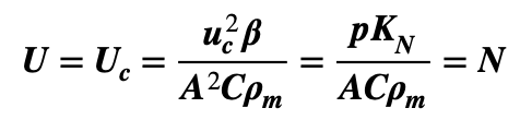
   We need to understand the boundary of the stable region where U < N and the limits of workable conditions for a system with U ≥ N. U = N .   gives critical current u_c and density j_c as follows:

   …202
   
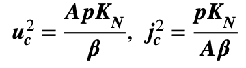
   …203
   

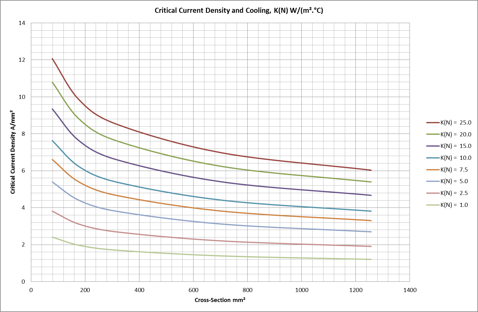
   Critical current and current-density values for copper are shown in Figs 05 & 06. 

   At the critical current, substituting the condition U = N = U_c  back into the CDE now gives:

   

   In this case, the substitution T = Z + at + b(x – x₀)² gives:

   

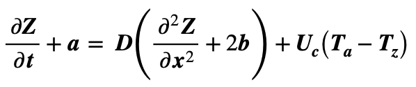
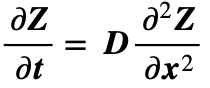
   If  a = 2Db + U_c(T_a – T_z) = 0  then the behaviour of Z is defined by the standard diffusion equation:
   
   

   Dispersion of the Z contribution is superposed upon the offset T₀ = at + b(x – x₀)² + c , with a b defined as above. In the simplest case of a uniform spatial distribution, Z = 0 and  b = 0 so that a = U_c(T_a – T_z) and temperature increases with a linear time dependence:
   

   

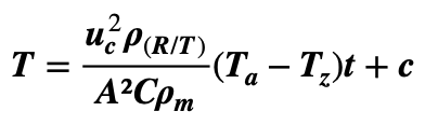
   Fig 05: Critical Current Values

   

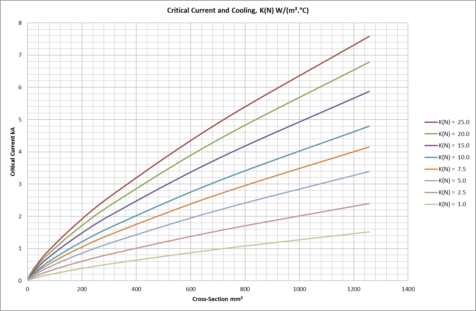
   Fig 06: Critical Current-Density Values

   

   High Current Density and Divergent Temperatures

   According to the analysis so far, temperature behaviour for (U ≠ N)  must satisfy the derived formula (106):

   

For each value of n the coefficients  w k satisfy the CSE:

As described above, with U < N , and K ~0, w < 0   and temperature converges towards equilibrium at  T = T_e. 

With (U = N), the CSE suggests w ≈ 0 with k ≈ 0  to give an inexorably linear temperature rise from near-zero exponent. 

Strictly, the situation at critical current  ( U = N = U_c ) invalidates the solutions applied for ( U ≠ N), but the linear offset in the proper solution fits neatly with solutions where ( U ≈ N ). Taking this onward, again with minimal spatial variation and k~0, then a positive value for ( U – N ) gives a positive exponent w t and the temperature diverges strongly. Fig 03, above, has already shown this type of exponential temperature trajectory. The concept of an equilibrium temperature is no longer valid but, for U ≫ N, (103) shows that the offset temperature T_e is given by T_e ≊ T_z.

In any case where ( U > N ), the CSE does reveal possible imaginary values for k which bring undulate spatial temperature distributions to (106) above. This now suggests exploration of complex values for both w and k as a response to imposed conditions

Complex Coefficients and Undulate Temperatures

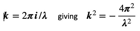
Undulate temperature conditions can be readily visualized by re-writing the CSE in the form:

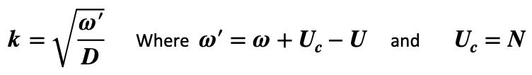
Whilst  U, N, D, relate to defined physical parameters and remain both real and positive, w k are exponential coefficients which may be real, imaginary or complex. The value of the spatial coefficient, k, can hence be pictured in an Argand diagram as a complex number derived from w’/D  with the square root of the modulus and half the argument. In 105 & 106 the formulae for temperature, temporal and spatial coefficients w and k provide real and imaginary contributions to the exponent. The sign and magnitude of the real components indicate rates of heat flux which determine whether the functions grow or shrink over time and distance. The imaginary contributions represent wave behaviour as combinations of temporal oscillation and spatial undulation.

Fig 07

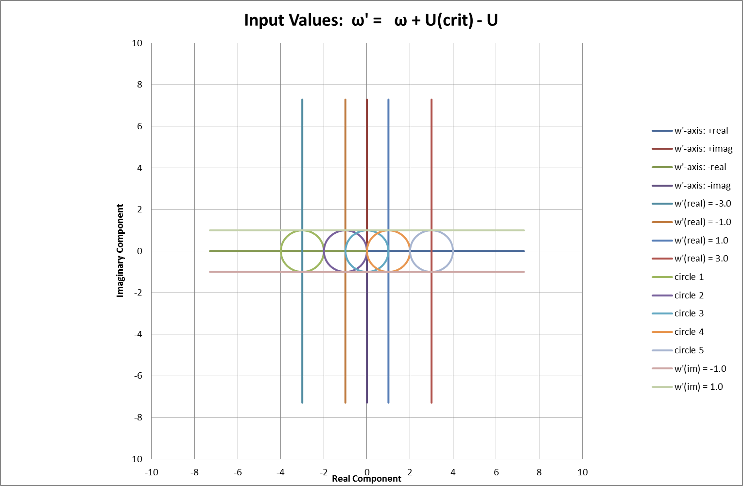
Fig 08

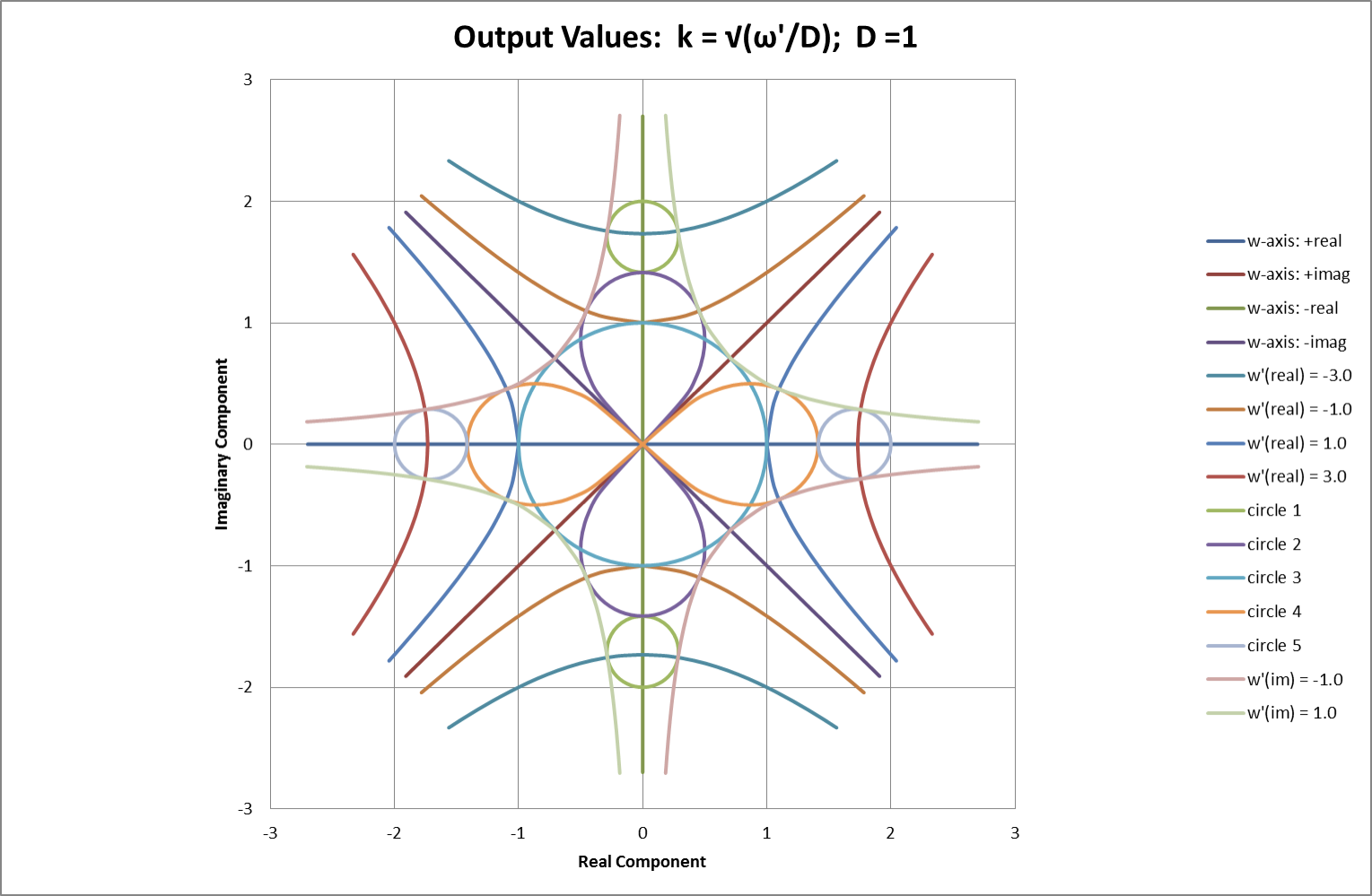
Figs 07 & 08 show corresponding Argand diagrams for w’ and k. Coloured lines represent points of constant real or constant imaginary value in Fig 07. Corresponding coloured pairs of hyperbolae represent the  +ve & -ve square root values of the same points in Fig 08. As a direct result of halving the argument in obtaining a square root, real and imaginary axes in the Fig 07 appear twice, at π/4 separation, in Fig 08. Vertical lines in the   plane represent constant current (strictly, constant U derived from the square of current). Horizontal lines represent a constant temporal oscillation frequency, f = w_imag/2π.

Fig 09: Wire Frame Model Representing Complex Wave-Numbers Shown in Fig 08

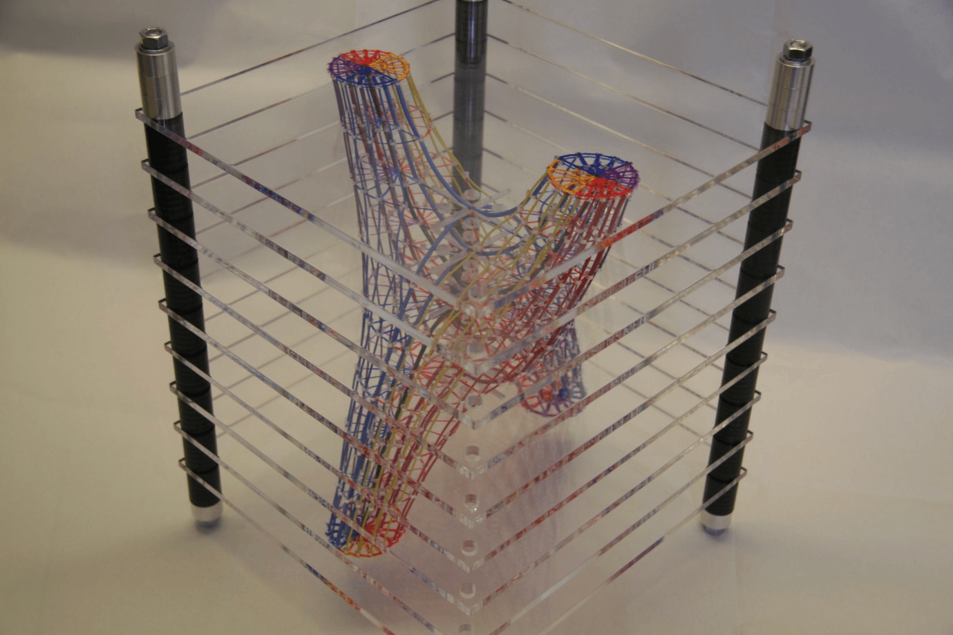
Fig 08 corresponds to looking directly downward onto the wire-frame model shown in Fig 09 but adds the axes transferred from Fig 07. Starting with circles representing variations in complex frequency, w, the model shows corresponding values of complex wavenumber, k , at various values of the rate-parameter, ( Uc – U ), principally determined by current. The plane of real axes in the above model runs from negative at the front LH centres to positive at the back-RH centres of each plane. Similarly, the plane of imaginary axes runs from front right to back left. 

Moving upwards through the planes represents increasing U by increasing current. U is real and has a minimum value zero. U_c is also a real rate parameter and represents the value of U equal to N, the rate parameter relating to cooling. The critical point, where U = Uc, corresponds to the circular centre of the form. Starting at U = 0, in the lower planes, values of k are centred on points on the real axis. Moving upwards through the centre and into the upper planes, where U > Uc  , values of k are centred on points on the imaginary axis.

The intersecting parabolae, corresponding to w = Dk2 + (U – N), are also visible within the structure of the model. Their central intersection, where U = U_c, corresponds to a break-over from real to imaginary values for k. On either side of the critical current this same break-over is offset by a spatial undulation according to the basic form of the CSE, here re-written as:

 A zero value for ω represents the break-over point in its transit from the negative values giving temporal stability to the instability arising from positive values. Spatial undulation, with wavelength λ, has a wave-number given by:

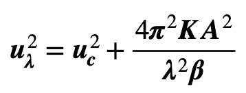
The condition w = 0 now gives a break-over value U = U_λ for undulation of a given wavelength:

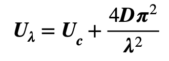
Using the values for u & D defined in (103) above, this enables a wavelength-dependent “cross-over current”, u_λ, to be evaluated as:

When transferred to the FEA model described later in the text, this formula accurately predicts the threshold value of current producing stability in an undulate temperature distribution. Currents below the threshold level, u_λ , allow the distribution to disperse whilst higher currents feed into the undulation, causing it to be amplified. The inverse-square dependence on wavelength provides a filtering effect that dissipates shorter wavelengths more rapidly owing to their higher “cross-over currents”. Referring back to 106, initial boundary conditions may comprise a temperature profile built up with a Fourier spectrum of undulation components. An example in the FEA results below shows how subsequent filtering can bias the spectrum toward the lower spatial frequencies. 

The complex planes and wire-frame model of Figs 07, 08 & 09 also show the range of possible phase relationships between the complex arguments for k and w. These are an important determinant of sustainable forms for undulation and oscillation. Careful inspection shows that co-incident non-zero wholly imaginary values for k and w are not possible. This precludes any possibility of “pure” travelling waves. The diagram shows that pure spatial undulation, without dispersion, only occurs when the imaginary component of w is zero. Lines of constant  w’_real  in Fig 07 show that imposed temporal oscillations, represented by variations in  w’_real , push the spatial undulation coefficient k shown in Fig 08 towards an asymptote of equal wavenumber and spatial attenuation rate (c.95% attenuation in one half-wavelength) represented by:

This prediction for forced oscillation is also in good quantitative agreement with the results of simulations in the FEA model that are described later.

Both formulae 303 & 305 above, plus the CSE, relate real values of measurable physical quantities (current, wavelength, resistivity etc.) by direct use of complex or imaginary values for the exponential coefficients  w  and k . Using complex numbers therefore provides a simple method to provide both variation and continuity in the linkage between dispersive and undulate behaviour. 

1. Advanced FEA Model
   

   Effect of Wavelength on Temperature Distribution

   Having seen the possibility of undulate temperature distributions, one of the first targets for the FEA model was an investigation of their stability. The model was set up with cylindrical zones whose length and diameter were determined by the required wavelength and conductor geometry. The LH termination reflected the temperature of the adjacent first zone and the RH termination connected to a virtual long cable with the same diameter as the model. An initial sinusoidal temperature distribution of one component frequency was then applied before iterations were run. To fit the characteristics of the model’s boundaries, 5/4 or 1/4 wavelengths were fitted with an antinode on the LH end and a node on the RH end. Results for 5/4 and ¼ wavelengths were found to be virtually identical. Typical results are shown below in Figs 10-12. 

   At any instant, the amplitude of the undulation was determined from the difference between measured maximum and minimum values. The rate of change of the natural logarithm of this number (gradient wrt time measured by linear regression) determined w_real  for the process with the relative time constant taken as its inverse. The current, u λ  , representing the break-over from attenuation to growth corresponds to the point where w_real  ≈ 0and iterative current adjustment enabled u_λ to be measured. Calculated values were then compared with these measurements, as shown in Table 01 below.

   Table 01: Comparison of Measured and Calculated Values for u_λ.

   λ	u λ	u λ	n λ(elected)
   Wavelength	Calculated	Measured	no. waves in model
   m	kA	kA	n
   0.8	6.307	6.309	5/4
   0.8	6.307	6.310	1/4
   4.0	2.393	2.393	5/4
   4.0	2.393	2.389	1/4
   20	2.090	2.090	5/4
   20	2.090	NA	1/4
   100	2.077	NA	5/4
   100	2.077	2.077	1/4

   Values for u_λ  and  u_c were calculated from both Eqn. 305 and Eqn. 203:

   

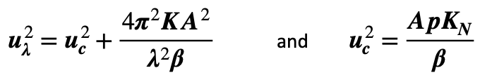
   Table 02: Parameter Values (cm-based) Used for Calculations.

   Attribute	Narrative	Value	Units
   K	Thermal Conductivity of Material (Cu)	4.00	Wcm¯¹°C¯¹
   A	Conductor Cross-Section Area	3.142	cm²
   β	(Lin) Resistivity Var’n with Temp.	6.867E-09	μΩcm°C¯¹
   p	Conductor perimeter	6.283	cm
   KN	(Elected) Newtonian Cooling Constant	15E-04	Wcm¯²°C¯¹
   (r)	Conductor Radius	1.00	cm
   	Calc. Critical Current (zero- )	2076	Amps

    

   Fig 10: Attenuated Undulation Amplitude, Conductor Critical Current = 2.076kA.

   

   

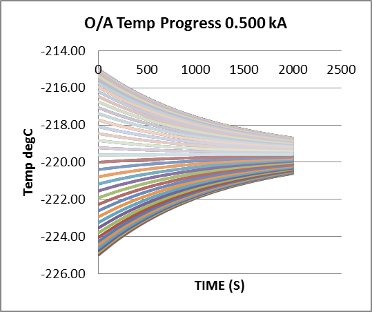
   Conductor current here is too low to sustain the initial undulate temperature distribution which therefore decays in amplitude, from 5degC to 0.95degC, over 2000s (33min). Over the same period, baseline temperature increases by 0.35degC.

   Both baseline starting temperature and ambient are set at -220degC.

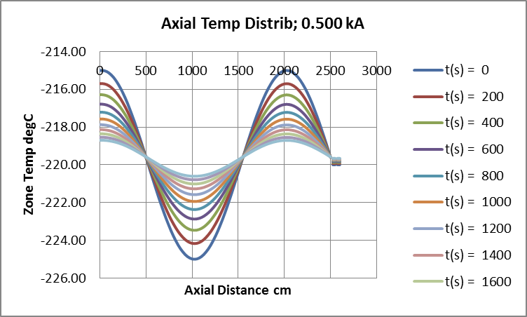
   Fig 11: Stable Undulation Amplitude, Conductor Critical Current = 2.076kA.

   

   

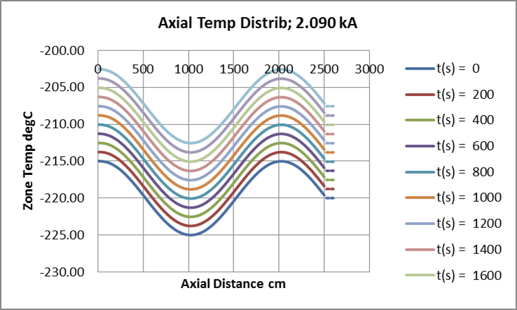
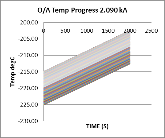
   The conductor current, u_λ, which just sustains an initial undulate temperature distribution has been found by iteration. Amplitude remains constant, at 5degC, over 2000s (33min). Over the same period, baseline temperature increases by 12.4degC at constant rate. 

   Both baseline starting temperature and ambient are set at -220degC.

   Fig 12: Divergent Undulation Amplitude, Conductor Critical Current = 2.076kA.

   

   

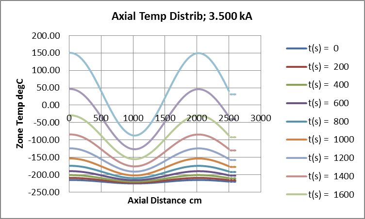
   Conductor current now feeds growth in the initial undulate temperature distribution which gains amplitude, from 5degC to 119degC, over 2000s (33min). Over the same period, baseline temperature increases exponentially by 251degC. 

   Both baseline starting temperature and ambient are set at -220degC.

   Temperature Distributions from Imposed Oscillation

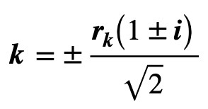
   Referring back to relationship between w and k defined by the CSE and shown in Figs 07-09, if the current is held at the critical value, u = u_c, then any imposed pure (constant amplitude) temperature oscillation results in a value for w’ that lies wholly on the imaginary axis (zero real-component). This should result in values for k limited to the form already described in Eqn. 306:

   

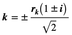
   Where the modulus, r_k, is given by the square root of the modulus, r’_w, of the complex value for w’. Any such temporal oscillation applied at the critical current should therefore result in spatial undulation with real and imaginary components sharing equal absolute values given by:

   

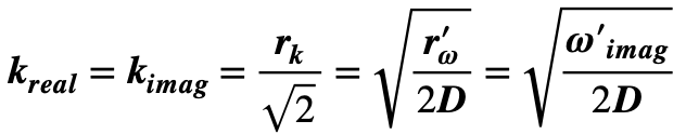
   Taking account of sign and direction, the attenuation distance-constant is given by d_Att = 1/k_real giving about 95% attenuation of amplitude over a distance d₉₅ ≅ 3 x d_Att. With spatial wave-length by λ = 2π/k_imag this represents heavy attenuation with only one half-wave effectively apparent.

   Response to oscillating-temperature was measured with essentially the same FEA model as that used for spatial undulation. The oscillation was super-imposed onto the bulk temperature and connected to one of the model’s end-terminations. As before, the other end-termination reflected the temperature of the adjacent zone.  Adjustment of the zone-length enabled model-length to be extended if significant temperature variations reached the reflection point during any set of iterations.  Attenuation of the applied temperature was again measured by linear regression applied to the logarithms of measured decay-distribution values, but it was now found necessary to allow the model several temperature cycles for the measurements to converge towards stability. Readings then corresponded to calculated values with reasonable accuracy. Although heavily attenuated, travelling wave-patterns emerging from the oscillator appear to need 10-50 cycles to stabilise themselves along the entire length of the model. Travel speeds, estimated from bulk-temperature differences for successive zones, coincided with the calculated values shown in Table 03 below.

   “Soft-starting” the simulations with linear amplitude increments for each full wave-cycle produced no faster approach to stability; increments on each half-cycle were not attempted. 

   For injected load-currents between zero and u_c  the temperature distribution would stabilise, exactly as described in the paragraphs above, to a heavily attenuated pattern effectively disappearing within one half-cycle, as shown in Fig 15, below.  Measurements and calculated values of decay distance-constant, corresponding to the real portion of the wave-number coefficient k, are again shown in Table 03 below. 

   Fig 13: GA Simulation and Bulk Measurements

   

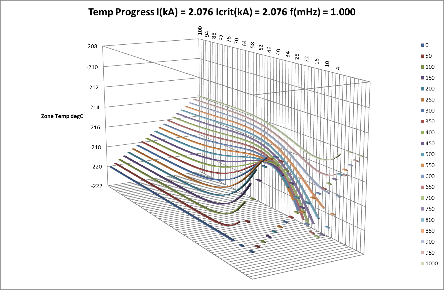
   Fig 14: GA Simulations and Difference Measurements

   

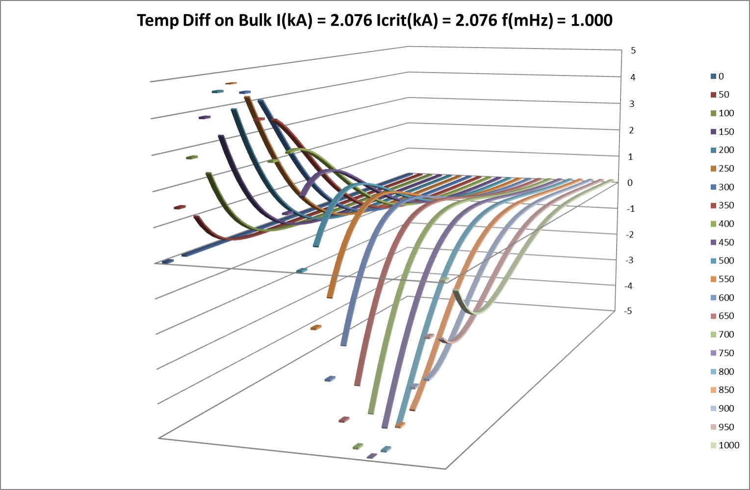
   Fig 15: Stable Response to Imposed Oscillation – Axial Differences on Bulk

   

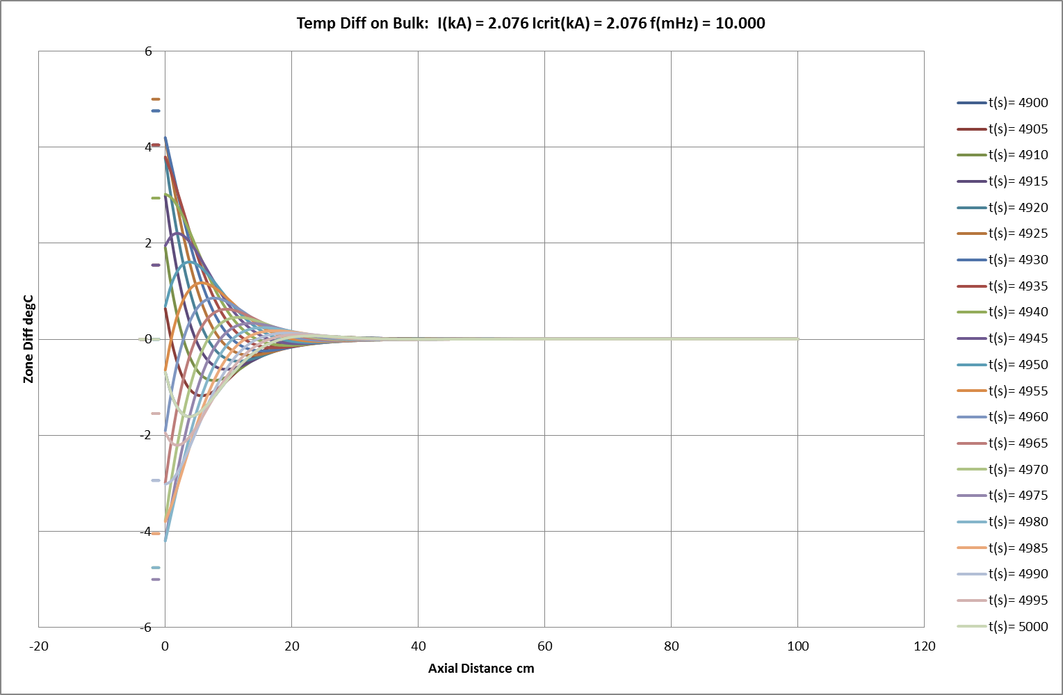
   Fig 16: Stable Response to Imposed Oscillation – Temporal Differences on Bulk

   

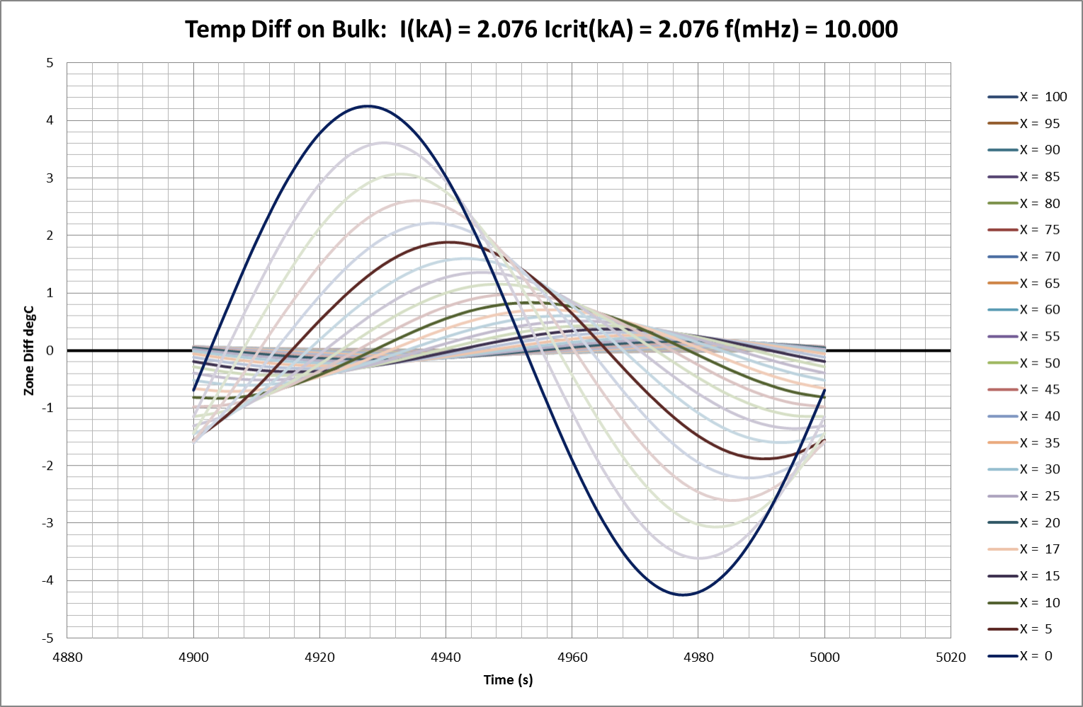
   Table 03: Imposed Temperature Oscillations (Conductor Critical Current, u_c , = 2.076kA)

   Selected FEA Results: Temp Oscillation Applied to Conductor
   Sim Ref	Ncycles	freq	Current	k(real) meas	k(real) calc	λ calc	v(wave) calc	NB
   		mHz	kA	cm¯¹	cm¯¹	cm	cm.sec¯¹
   C7	50	1.0	2.076	-0.0523	-0.0524	120.5	0.120	stable
   C22	20	1.0	2.200	-0.0523	-0.0517	119.4	0.119
   C25	20	1.0	2.300	-0.0549	-0.0514	118.6	0.119
   C26	6	1.0	2.500	-0.0490	-0.0506	116.8	0.117
   C27	3	1.0	3.000	-0.0403	-0.0484	111.8	0.112
   C10	50	2.0	2.076	-0.0740	-0.0740	85.2	0.170	stable
   C29	50	10.0	2.076	-0.1627	-0.1650	38.1	0.381	stable
   C30	1	10.0	10.000	-0.1138	-0.1419	32.8	0.328	Fig 17a
   C31	2	10.0	10.000	-0.0620	-0.1419	32.8	0.328	Fig 17b
   C32	3	10.0	10.000	0.0593	-0.1419	32.8	0.328	Fig 17c
   C11	20	100.0	0.000	-0.5134	-0.5220	12.1	1.205	stable
   C13	41	100.0	2.076	-0.5131	-0.5217	12.0	1.204	stable
   C14	20	100.0	4.000	-0.5123	-0.5207	12.0	1.202
   C18	20	100.0	10.000	-0.4887	-0.5137	12.0	1.202
   C19	3	100.0	20.000	-0.4060	-0.4897	11.3	1.131

   Instability in Undulation Induced by Oscillation

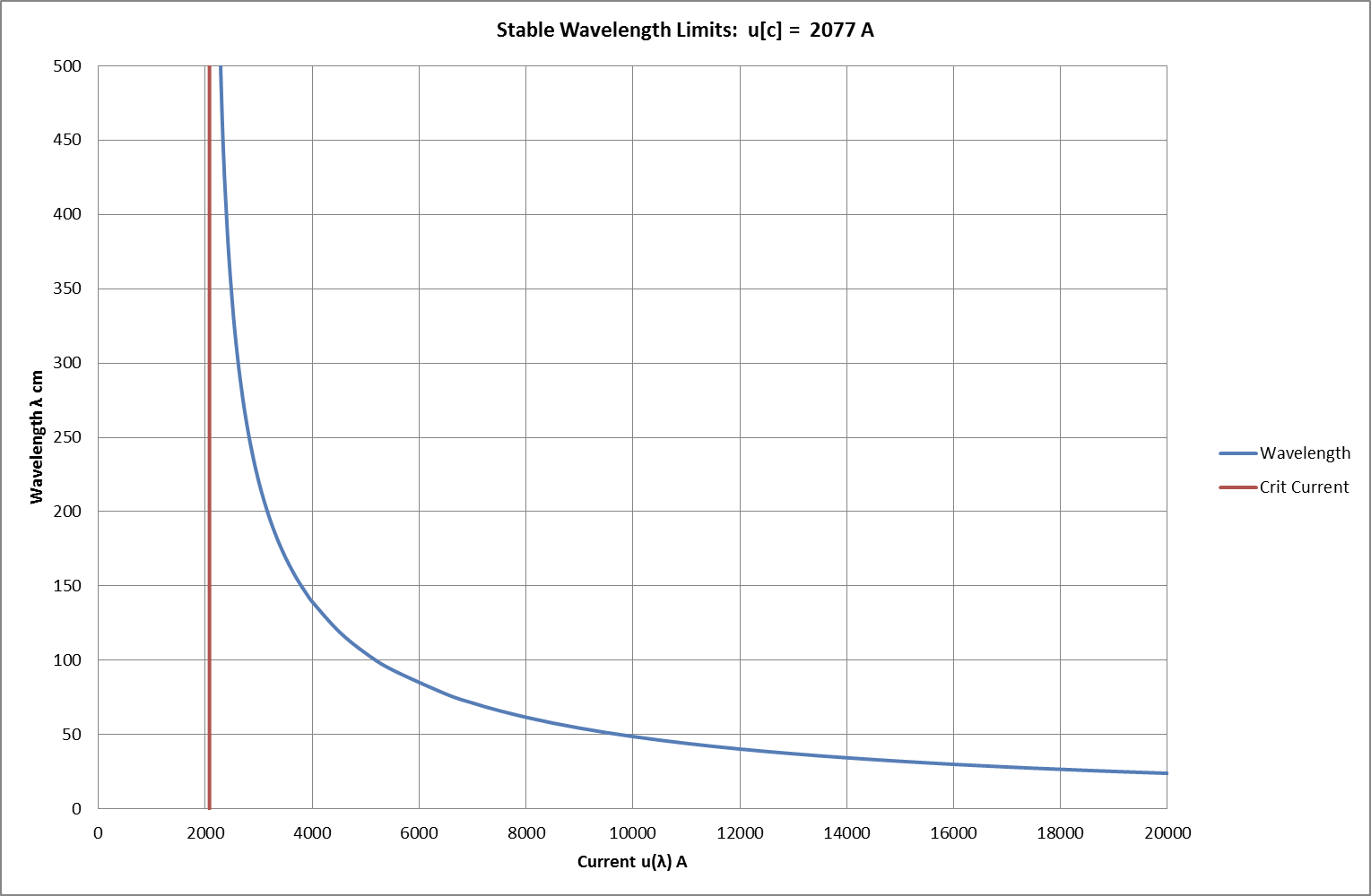
   Increasing the injected current beyond u_c will eventually cause the temperature wave-distribution to become unstable. The typical pattern is shown in Figs 17a-d where it can be seen that the injected current causes the same rapid growth or amplification described earlier for static waves. Fig 18 shows an extended range of “break-over” current and corresponding critical wavelengths as calculated in the earlier section on stability of undulate spatial distributions. It predicts that 10kA injected into a conductor with critical current 2kA would support or enhance undulate distributions with a wavelength longer than about 50cm (calc: 48.71cm). In the illustrated sequence, a 10mHz temperature oscillation of 5°C is imposed on a conductor (with u_c = 2.076kA) carrying 10kA current. This initiates a heavily-attenuated travelling wave with calculated wavelength of 32.75 cm and attenuation coefficient of negative0.14cm¯¹ (=> halving in 5.0cm); measured as reasonably accurate over the first part of the modelled 100cm. Instability then develops however and attenuation progresses from negative (-0.11cm¯¹ =>halving in 6.3cm) to positive (+0.06cm¯¹ => doubling in 11.6cm) and wavelength visibly increases to ITRO the predicted 50cm minimum.

   In basic terms, an oscillating thermal disturbance at the end of the conductor develops into a singularity with minimum viable half-wavelength for the applied current-level.

   Fig 17a: Emergent Instability with Load Current Exceeding Critical Value ( u_c )

   

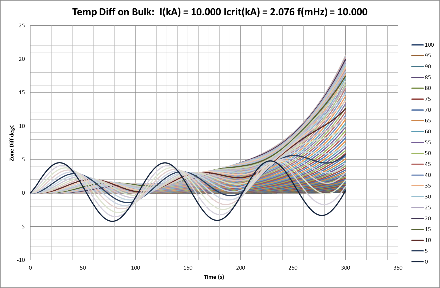
   Fig 17b: Emergent Instability with Load Current Exceeding Critical Value ( u_c )

   

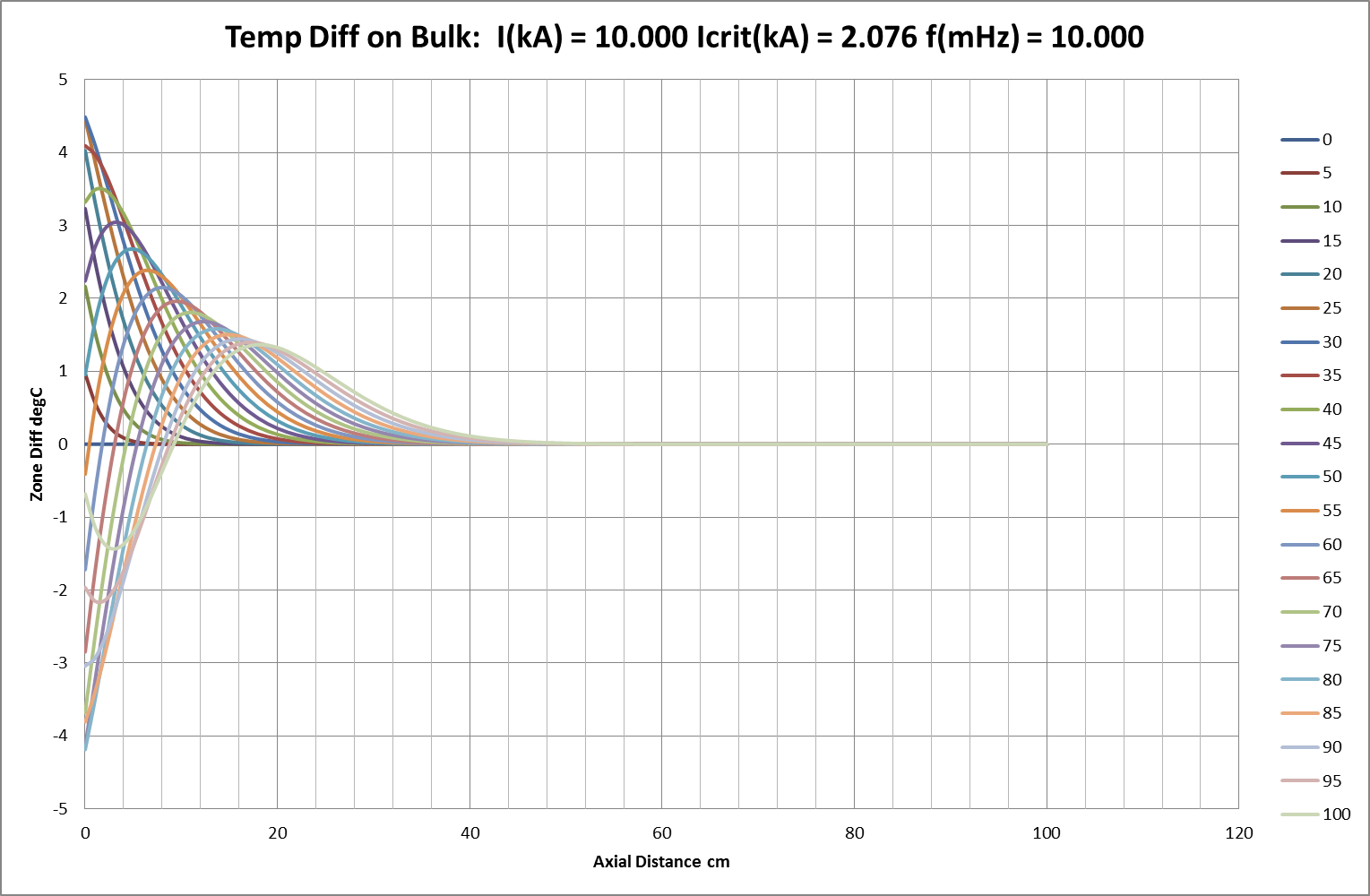
   Fig 17c: Emergent Instability with Load Current Exceeding Critical Value ( u_c )

   

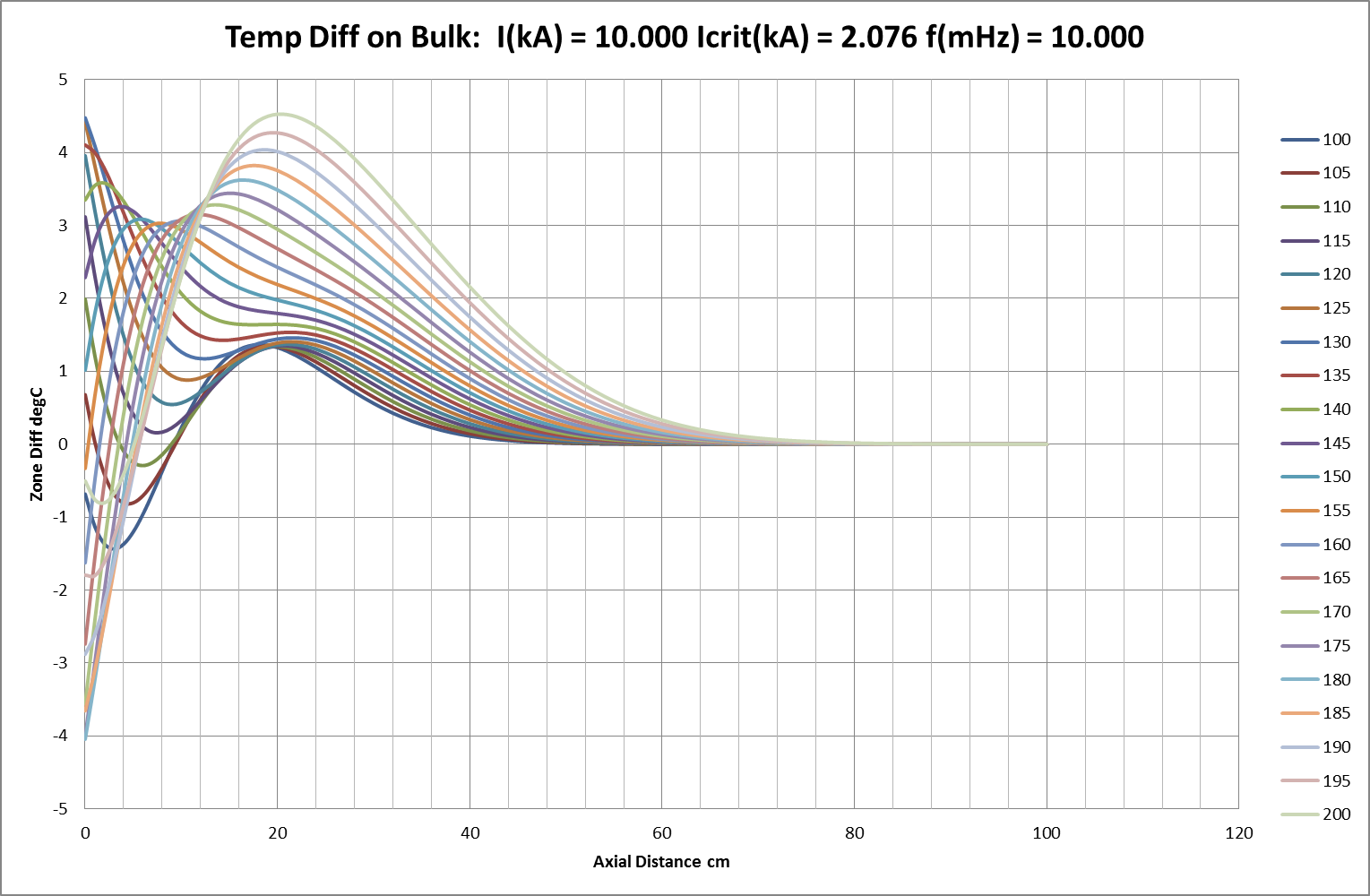
   Fig 17d: Emergent Instability with Load Current Exceeding Critical Value ( u_c )

   

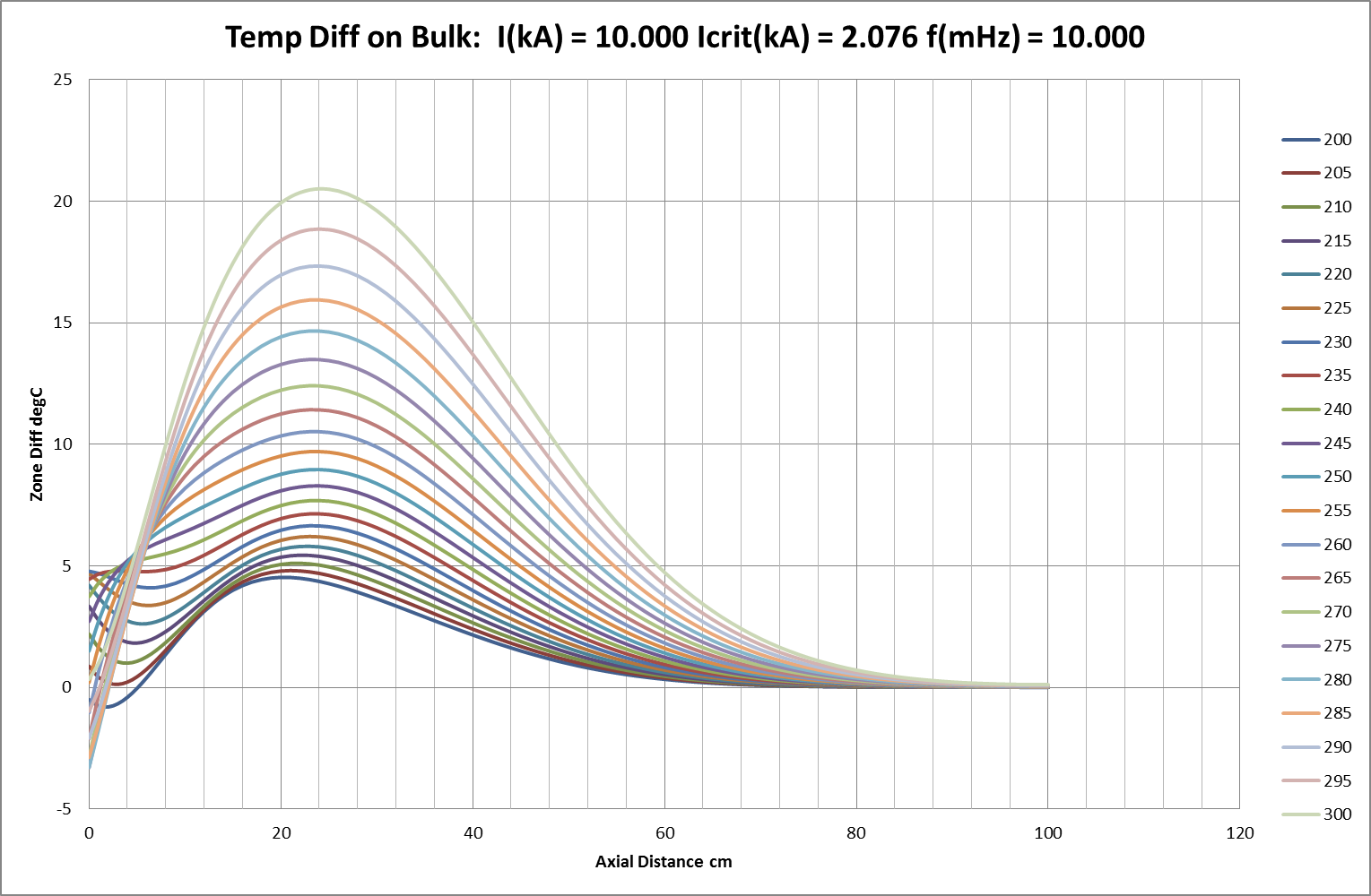
   Fig 18: Current Limits for Stable Static Undulation, Critical Current = 2.08kA

   

2. Conclusions

   The results measured from FEA modelling of conductors show good agreement with the predictions of the mathematical model represented by the construction of the Central Differential Equation and its solutions. Given adequate data, practical arrangements of conductors and boundary conditions can therefore be examined in detail, or potentially validated, using results from these types of modelling and analysis. A more complex model would be required to accommodate trans-axial variations in conductor temperature, but the essential techniques would remain the same.

   The models outline the conditions for two basic types of behaviour:

   1. Stable conditions under modest loads with an axial distribution of equilibrium temperatures to which the system reverts after temporary, localised displacement.
   2. Unstable conditions under extreme loads where overall temperatures increase exponentially and where spatially-distributed temperature singularities and differences are exacerbated. Unchecked, this leads to localised points of destructive failure.